Jpeg: Colorspace Transform, Subsampling, DCT and Quantisation

In this document the first 4 steps of the JPEG encoding chain are demonstrated. These 4 steps contain the lossy parts of the coding. The remaining steps, i.e. runlength and Huffman encoding, are losless. Therefore the 4 steps demonstrated here are sufficient to study the quality-loss of JPEG encoding.

The following packages are required.:

import cv2
import numpy as np
from matplotlib import pyplot as plt
import matplotlib.cm as cm

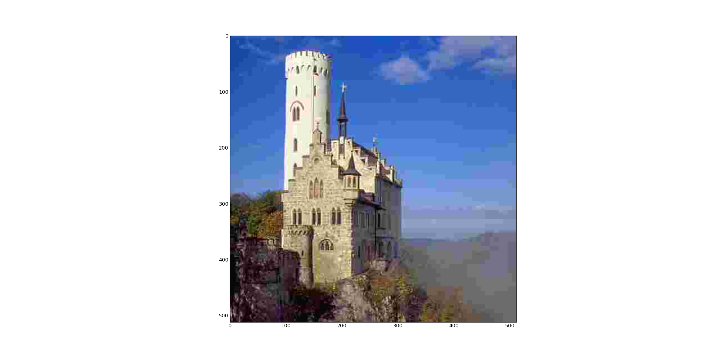
Step 1: Read and display image

In OpenCV color images are imported as BGR. In order to display the image with pyplot.imshow() the channels must be switched such that the order is RGB.:

B=8 # blocksize (In Jpeg the
img1 = cv2.imread("lichtenstein.png", cv2.CV_LOAD_IMAGE_UNCHANGED)
h,w=np.array(img1.shape[:2])/B * B
img1=img1[:h,:w]
#Convert BGR to RGB
img2=np.zeros(img1.shape,np.uint8)
img2[:,:,0]=img1[:,:,2]
img2[:,:,1]=img1[:,:,1]
img2[:,:,2]=img1[:,:,0]
plt.imshow(img2)

The user is asked to click into the image. The clicked block is highlighted in the image (blue rectangle). For the clicked block the DCT coefficients will be displayed later:

point=plt.ginput(1)
block=np.floor(np.array(point)/B) #first component is col, second component is row
print "Coordinates of selected block: ",block
scol=block[0,0]
srow=block[0,1]
plt.plot([B*scol,B*scol+B,B*scol+B,B*scol,B*scol],[B*srow,B*srow,B*srow+B,B*srow+B,B*srow])
plt.axis([0,w,h,0])

Step 2: Transform BGR to YCrCb and Subsample Chrominance Channels

Using OpenCV the color space transform is implemented by:

transcol=cv2.cvtColor(img1, cv2.cv.CV_BGR2YCrCb)

Next, the chrominance channels Cr and Cb are subsampled. The constant SSH defines the subsampling factor in horicontal direction, SSV defines the vertical subsampling factor. Before subsampling the chrominance channels are filtered using a (2x2) box filter (=average filter). After subsampling all 3 channels are stored in the list imSub:

SSV=2
SSH=2
crf=cv2.boxFilter(transcol[:,:,1],ddepth=-1,ksize=(2,2))
cbf=cv2.boxFilter(transcol[:,:,2],ddepth=-1,ksize=(2,2))
crsub=crf[::SSV,::SSH]
cbsub=cbf[::SSV,::SSH]
imSub=[transcol[:,:,0],crsub,cbsub]

Step 3 and 4: Discrete Cosinus Transform and Quantisation

First the quantisation matrices for the luminace channel (QY) and the chrominance channels (QC) are defined, as proposed in the annex of the Jpeg standard.:

QY=np.array([[16,11,10,16,24,40,51,61],
                         [12,12,14,19,26,48,60,55],
                         [14,13,16,24,40,57,69,56],
                         [14,17,22,29,51,87,80,62],
                         [18,22,37,56,68,109,103,77],
                         [24,35,55,64,81,104,113,92],
                         [49,64,78,87,103,121,120,101],
                         [72,92,95,98,112,100,103,99]])

QC=np.array([[17,18,24,47,99,99,99,99],
                         [18,21,26,66,99,99,99,99],
                         [24,26,56,99,99,99,99,99],
                         [47,66,99,99,99,99,99,99],
                         [99,99,99,99,99,99,99,99],
                         [99,99,99,99,99,99,99,99],
                         [99,99,99,99,99,99,99,99],
                         [99,99,99,99,99,99,99,99]])

In order to provide different quality levels a quality factor QF can be selected. From the quality factor the scale parameter is calculated. The matrices defined above are multiplied by the scale parameter. A low quality factor implies are large scale parameter. A large scale parameter yields a coarse quantisation, a low quality but a high compression rate. The list Q contains the 3 scaled quantisation matrices, which will be applied to the DCT coefficients:

QF=99.0
if QF < 50 and QF > 1:
        scale = np.floor(5000/QF)
elif QF < 100:
        scale = 200-2*QF
else:
        print "Quality Factor must be in the range [1..99]"
scale=scale/100.0
Q=[QY*scale,QC*scale,QC*scale]

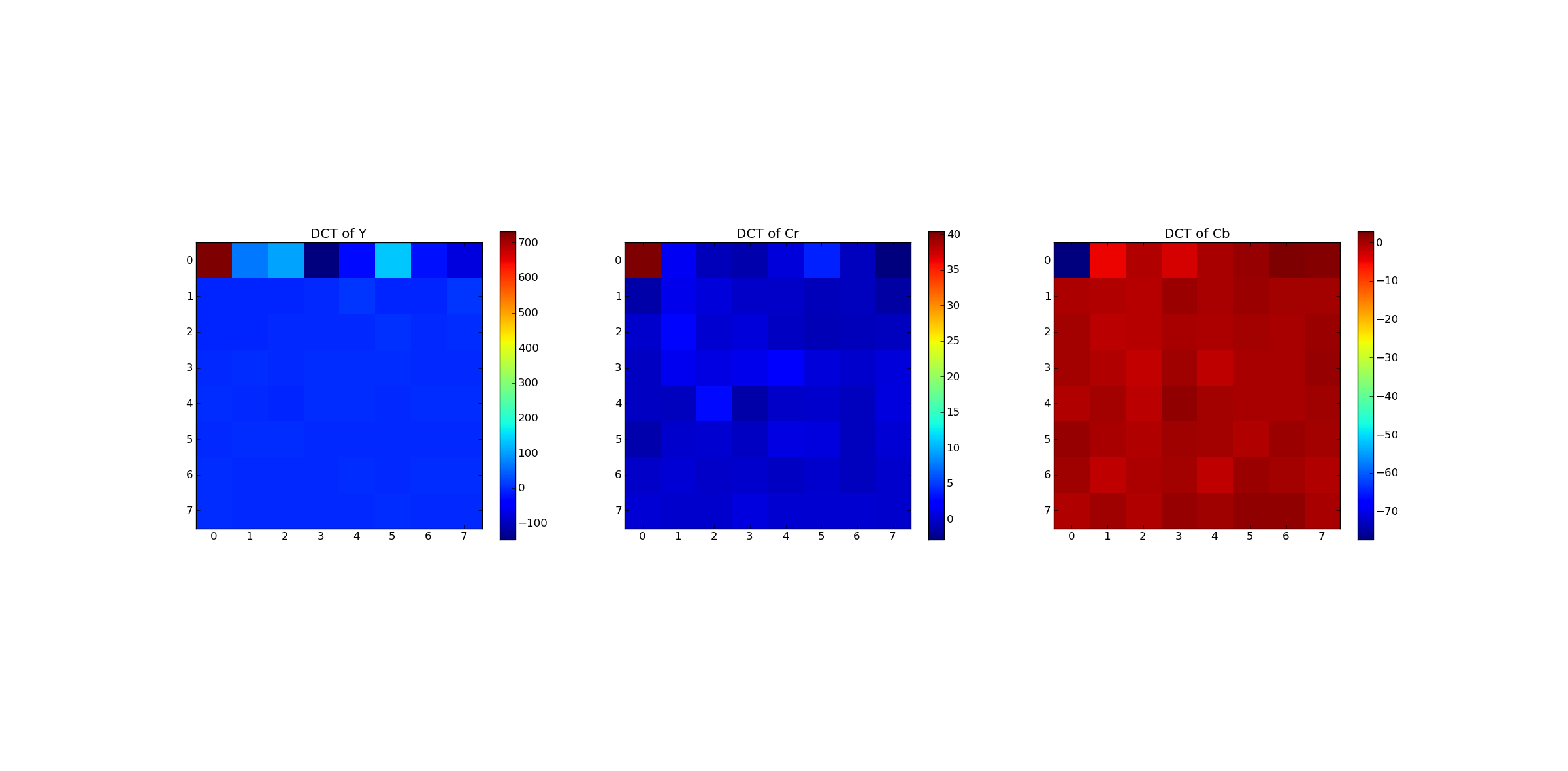
In the following loop DCT and quantisation is performed channel by channel. As defined in the standard, before DCT the pixel values of all channels are shifted by -128, such that the new value range is [-128,...127]. The loop iterates over the imSub-list, which contains the 3 channels. The result of the DCTs of the 3 channels are stored in 2-dimensional numpy arrays, which are put into the python list TransAll. Similarly the quantized DCT coefficients are stored in 2-dimensional numpy arrays, which are assigned to the python list TransAllQuant. Note that the channels have different shapes due to chrominance subsampling. In the last part of the loop the DCT coefficients of the previously selected and highlighted block are displayed:

TransAll=[]
TransAllQuant=[]
ch=['Y','Cr','Cb']
plt.figure()
for idx,channel in enumerate(imSub):
        plt.subplot(1,3,idx+1)
        channelrows=channel.shape[0]
        channelcols=channel.shape[1]
        Trans = np.zeros((channelrows,channelcols), np.float32)
        TransQuant = np.zeros((channelrows,channelcols), np.float32)
        blocksV=channelrows/B
        blocksH=channelcols/B
        vis0 = np.zeros((channelrows,channelcols), np.float32)
        vis0[:channelrows, :channelcols] = channel
        vis0=vis0-128
        for row in range(blocksV):
                for col in range(blocksH):
                        currentblock = cv2.dct(vis0[row*B:(row+1)*B,col*B:(col+1)*B])
                        Trans[row*B:(row+1)*B,col*B:(col+1)*B]=currentblock
                        TransQuant[row*B:(row+1)*B,col*B:(col+1)*B]=np.round(currentblock/Q[idx])
        TransAll.append(Trans)
        TransAllQuant.append(TransQuant)
        if idx==0:
                selectedTrans=Trans[srow*B:(srow+1)*B,scol*B:(scol+1)*B]
        else:
                sr=np.floor(srow/SSV)
                sc=np.floor(scol/SSV)
                selectedTrans=Trans[sr*B:(sr+1)*B,sc*B:(sc+1)*B]
        plt.imshow(selectedTrans,cmap=cm.jet,interpolation='nearest')
        plt.colorbar(shrink=0.5)
        plt.title('DCT of '+ch[idx])

Decoding

In order to show the quality decrease caused by the Jpeg coding the 4 steps performed above are inverted in order to decode the image. In the following loop for each channel first the inverse quantisation is performed, followed by the inverse dct and the inverse shiftign of the shift of the pixel values, sucht that their value range is [0,...,255]. Moreover the subsampled chrominance channels are interpolated, using the opencv method resize() such that their original size is reconstructed.:

DecAll=np.zeros((h,w,3), np.uint8)
for idx,channel in enumerate(TransAllQuant):
        channelrows=channel.shape[0]
        channelcols=channel.shape[1]
        blocksV=channelrows/B
        blocksH=channelcols/B
        back0 = np.zeros((channelrows,channelcols), np.uint8)
        for row in range(blocksV):
                for col in range(blocksH):
                        dequantblock=channel[row*B:(row+1)*B,col*B:(col+1)*B]*Q[idx]
                        currentblock = np.round(cv2.idct(dequantblock))+128
                        currentblock[currentblock>255]=255
                        currentblock[currentblock<0]=0
                        back0[row*B:(row+1)*B,col*B:(col+1)*B]=currentblock
        back1=cv2.resize(back0,(h,w))
        DecAll[:,:,idx]=np.round(back1)

The 3-dimensional numpy-array DecAll contains the decoded YCrCb image. This image is backtransformed to BGR, stored to a file and displayed in a pyplot figure. Finally the Sum of squared error (SSE) between the original image and the decoded image is calculated:

reImg=cv2.cvtColor(DecAll, cv2.cv.CV_YCrCb2BGR)
cv2.cv.SaveImage('BackTransformedQuant.jpg', cv2.cv.fromarray(reImg))
plt.figure()
img3=np.zeros(img1.shape,np.uint8)
img3[:,:,0]=reImg[:,:,2]
img3[:,:,1]=reImg[:,:,1]
img3[:,:,2]=reImg[:,:,0]
plt.imshow(img3)
SSE=np.sqrt(np.sum((img2-img3)**2))
print "Sum of squared error: ",SSE
plt.show()

The SSE for different quality factors and subsampling schemes is displayed in the table below.

Subsampling	Quality Factor	SSE
4:2:0	10	6330
4:2:0	40	4740
4:2:0	70	4170
4:2:0	99	2545
4:4:4	99	1885

The following images demonstrate the quality decrease with decreasing quality factor QF.

Subsampling 4:2:0, Quality Factor QF=10

Subsampling 4:2:0, Quality Factor QF=40

Subsampling 4:2:0, Quality Factor QF=70