Information Theory
For a general Python introduction see e.g. Python Introduction.
Calculate Entropy of Text
The entropy of a given sequence of symbols constitutes a lower bound on the average number of bits required to encode the symbols. In the case that the symbol sequence is a text the entropy can be calculated as below. The imported package Numpy is the fundamental package for scientific computing with Python.:
import numpy as np
text="""In agreeing to settle a case brought by 38 states involving the project, the search company for the first time is required to aggressively police its own employees on privacy issues and to explicitly tell the public how to fend off privacy violations like this one."""
chars=list(text)
length=len(chars)
print "Number of characters in text string: %d"%(length)
dec=[ord(c) for c in chars]
decset=set(dec)
In the code snippet above the text, contained in a single string variable, is converted into a list of characters. The length of the message in characters is calculated and printed to the console. Then for the given list of characters the corresponding list of deciaml numbers, according to the ASCII code is calculated. This step is actually not necessary for the entropy calculation. It just serves to demonstrate how characters can be converted to their decimal ascii representation. The variable decset contains the set of all characters, that occur in the text.
In the code snippet below a dictionary freqdict is created, whose keys are the decimal representations of all characters that occur in the text. The values are the frequency counts for the corresponding character. In the succeeding for loop for each character the probability and the information content of this character in the text is calculated. The entropy is then calculated as the sum over all products of character probability and character information content.:
freqdic={}
for c in decset:
        freqdic[c]=dec.count(c)

print "\nAscii \t Char \t Count \t inform."
Entropy=0
for c in decset:
        prop=freqdic[c]/(1.0*length) #propability of character
        informationContent=np.log2(1.0/prop) #infromation content of character
        Entropy+=prop*informationContent
        print "%5d \t %5s \t %5d \t %2.2f" %(c, chr(c),freqdic[c],informationContent)

print "\nEntropy of text: %2.2f"%(Entropy)
Calculate Entropy of Image
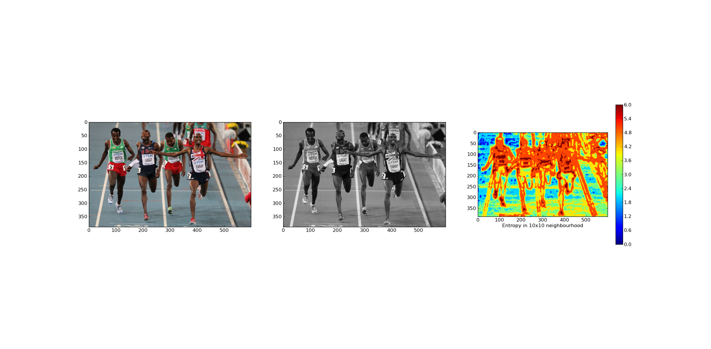
The entropy of an image can be calculated by calculating at each pixel position (i,j) the entropy of the pixel-values within a 2-dim region centered at (i,j). In the following example the entropy of a grey-scale image is calculated and plotted. The region size is configured to be (2N x 2N) = (10,10).
Besides Numpy the imported packages are PIL and Matplotlib. The Python Imaging Library (PIL) provides standard image processing functions, e.g. for filtering and transcoding. Matplotlib is a python 2D plotting library.:
from PIL import Image
import numpy as np
from matplotlib import pyplot as plt
The function entropy takes a 1-dimensional array and calculates the entropy of the symbols in the array.:
def entropy(signal):
        '''
        function returns entropy of a signal
        signal must be a 1-D numpy array
        '''
        lensig=signal.size
        symset=list(set(signal))
        numsym=len(symset)
        propab=[np.size(signal[signal==i])/(1.0*lensig) for i in symset]
        ent=np.sum([p*np.log2(1.0/p) for p in propab])
        return ent
A jpeg image is loaded and a grey-scale copy of this image is generated. For further processing the PIL-images are converted to numpy-arrays.:
colorIm=Image.open('mo.JPG')
greyIm=colorIm.convert('L')
colorIm=np.array(colorIm)
greyIm=np.array(greyIm)
The parameter N defines the size of the region within which the entropy is calculated. For N=5 the region contains 10*10=100 pixel-values. In the following loop for each pixel position the corresponding neighbour region is extracted. The 2-dimensional neighbourhood is flattened into a 1-dimensional numpy array and passed to the entropy function. The entropy values are inserted into the entropy-array E.:
N=5
S=greyIm.shape
E=np.array(greyIm)
for row in range(S[0]):
        for col in range(S[1]):
                Lx=np.max([0,col-N])
                Ux=np.min([S[1],col+N])
                Ly=np.max([0,row-N])
                Uy=np.min([S[0],row+N])
                region=greyIm[Ly:Uy,Lx:Ux].flatten()
                E[row,col]=entropy(region)
Finally the original RGB image, the corresponding grey-scale image and the entropy image are plotted using matplotlib’s pyplot function.:
plt.subplot(1,3,1)
plt.imshow(colorIm)

plt.subplot(1,3,2)
plt.imshow(greyIm, cmap=plt.cm.gray)

plt.subplot(1,3,3)
plt.imshow(E, cmap=plt.cm.jet)
plt.xlabel('Entropy in 10x10 neighbourhood')
plt.colorbar()

plt.show()
As the entropy image shows homogenous regions have low entropy.
Comparison and Evaluation
Objective and subjective comparison of images
The PIL package is applied for transcoding images. A uncoded bitmap bmp is loaded into the program and saved as .jpg- and as .png-image.:
from PIL import Image
import numpy as np
from matplotlib import pyplot as plt


bmpIm=Image.open('Bretagne32.bmp')
bmpIm.save('Bretagne.jpg')
bmpIm.save('Bretagne.png')
bmpIm=np.array(bmpIm)
The encoded .jpg- and .png-images are then loaded into the program and the root mean square error (rmse) between each possible pair of images is calculated.:
jpgIm=Image.open('Bretagne.jpg')
jpgIm=np.array(jpgIm)
pngIm=Image.open('Bretagne.png')
pngIm=np.array(pngIm)
msebj=np.sqrt(np.sum((bmpIm-jpgIm)**2))
print msebj
msebp=np.sqrt(np.sum((bmpIm-pngIm)**2))
print msebp
msejp=np.sqrt(np.sum((pngIm-jpgIm)**2))
print msejp
What do you expect for the 3 rmse values? What are the sizes of the 3 image files? Finally, the 3 image versions are plotted into one matplotlib figure. Are there any subjective differences?.:
plt.subplot(1,3,1)
plt.imshow(bmpIm)
plt.title("Bitmap")

plt.subplot(1,3,2)
plt.imshow(jpgIm)
plt.title("Jpeg")

plt.subplot(1,3,3)
plt.imshow(pngIm)
plt.title("Png")
plt.show()
