Color Space Transformations

RGB to YcrCb conversion

OpenCV provides methods to convert between the most common color spaces. In this section only the conversion from RGB to YCrCb is demonstrated.

The following packages must be imported:

import cv2
import numpy as np
from matplotlib import pyplot as plt

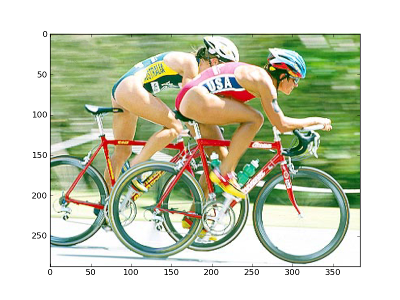
A RGB color image is imported. The returned numpy-array is 3-dimensional, i.e. one 2-dimensional array per color channel:

fn3= 'tria.jpg'
img1 = cv2.imread(fn3, cv2.CV_LOAD_IMAGE_UNCHANGED)

Note that in OpenCV RGB images are represented as BGR. Thus the first component img[:,:,0] is the blue channel and the last component img[:,:,2] is the red channel. In order to display the color image using Pyplot’s imshow() method, a copy of image img1 is generated, which contains the color channels in the usual order RGB.:

img2=np.zeros(img1.shape,np.uint8)
img2[:,:,0]=img1[:,:,2]
img2[:,:,1]=img1[:,:,1]
img2[:,:,2]=img1[:,:,0]
plt.imshow(img2)

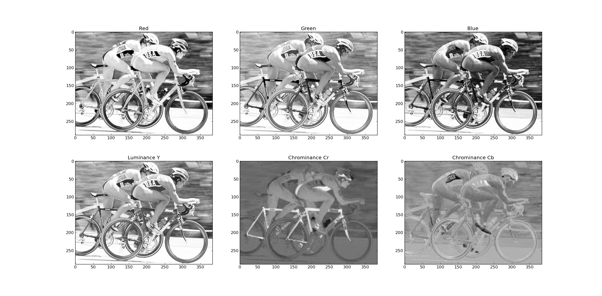
Next the BGR image is converted into a YCrCb image:

transcol=cv2.cvtColor(img1, cv2.cv.CV_BGR2YCrCb)

The RGB channels and the YCrCb channels are plotted in a single pyplot figure as intensity images.:

plt.figure()
plt.subplot(2,3,1)
plt.imshow(img1[:,:,2],cmap="gray")
plt.title('Red')
plt.subplot(2,3,2)
plt.imshow(img1[:,:,1],cmap="gray")
plt.title('Green')
plt.subplot(2,3,3)
plt.imshow(img1[:,:,0],cmap="gray")
plt.title('Blue')

plt.subplot(2,3,4)
plt.imshow(transcol[:,:,0],cmap="gray")
plt.title('Luminance Y')
plt.subplot(2,3,5)
plt.imshow(transcol[:,:,1],cmap="gray")
plt.title('Chrominance Cr')
plt.subplot(2,3,6)
plt.imshow(transcol[:,:,2],cmap="gray")
plt.title('Chrominance Cb')
plt.show()

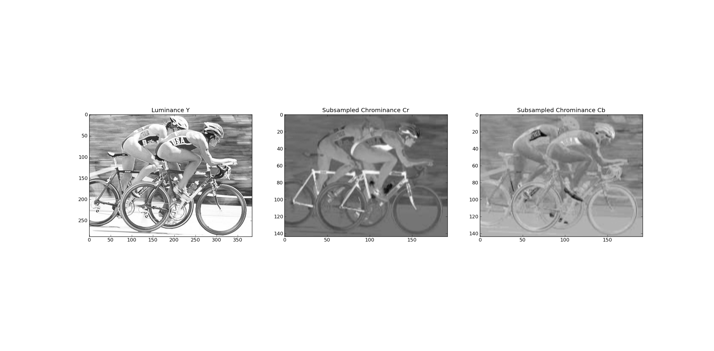
Subsampling of Chrominance Channels

The YCrCb color space is used, because the human eyes are less sensitive to chrominance changes than to luminance changes. Hence the chrominance channels can be subsampled in a lossy compression procedure. If the following code snippet is attached to the code described above, the chrominance channels are first filtered with a box filter of size (2,2). The filtered subchannels are then subsampled by a factor of 2 in both, the vertical and the horicontal direction. This yields a compression of the entire image (all 3 channels) by a factor of 2.:

crf=cv2.boxFilter(transcol[:,:,1],ddepth=-1,ksize=(2,2))
cbf=cv2.boxFilter(transcol[:,:,2],ddepth=-1,ksize=(2,2))
print type(crf[0,0])
SSV=2
SSH=2
crsub=crf[::SSV,::SSH]
cbsub=cbf[::SSV,::SSH]

The subsampled channels are plotted as follows:

plt.figure()
plt.subplot(1,3,1)
plt.imshow(transcol[:,:,0],cmap="gray")
plt.title('Luminance Y')
plt.subplot(1,3,2)
plt.imshow(crsub,cmap="gray")
plt.title('Subsampled Chrominance Cr')
plt.subplot(1,3,3)
plt.imshow(cbsub,cmap="gray")
plt.title('Subsampled Chrominance Cb')
plt.show()